-
Notifications
You must be signed in to change notification settings - Fork 2
Concepts
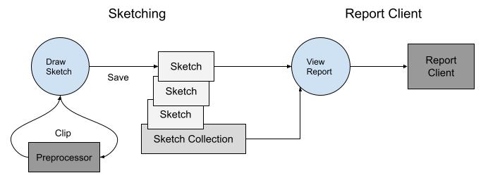
A SeaSketch planning process typically does the following:

- Captures user input in the form of spatial features (sketches) with attributes (e.g. allowed activities, notes, etc.). Sketches are then organized into proposals (sketch collections).
- Provides feedback (reports) on how well sketches and sketch collections meet measurable planning objectives and their targets (using geoprocessing functions).
- Users then share and iterate on their designs until the group together can make proposals, narrow them down, and come to a decision.
The project goal is met if all measurable objectives are met and the proposal is legally viable.
The core SeaSketch platform is designed to accomplish #1 and #3. The geoprocessing framework is primarily used to accomplish #2, as well as #1 (using preprocessing functions). The two systems work together to provide an end-to-end spatial planning solution.
What's unique about the geoprocessing framework is it's flexibility. It's not one-size-fits-all. A developer can create custom reports through code starting with a template.
A geoprocessing project starts with a design phase, using a planning tool design template.
There are a number of terms and concepts to be familiar with:
-
MPA- [marine protected area]. Protected areas of seas, oceans, estuaries. (https://en.wikipedia.org/wiki/Marine_protected_area) -
Goal- also known as vision or aim. These are general summaries of the desired future state of an area.- Example - Protect biological diversity, productivity, and ecological function across all habitat types
-
Objective- aka purpose. These are specific statements that describe how the goal will be reached and are typically measurable or quantifiable in some way.- Example - Designate a minimum of 20% of the EEZ as fully protected no-take Marine Protected Areas.
-
Target- The measurement to reach to say that an objective has been met.- Example - 20% of the EEZ
One or more Geographies are then defined that define the planning boundaries for the project. This can be one large overarching boundary for the project, and/or multiple smaller planning boundaries.
Datasources are then created/gathered to defined the extent of each Geography, and to provide data that measures progress towards an objective. For example:
- A polygon boundary of a countries Exclusive Economic Zone is used to measure what % of the EEZ a proposed area covers.
- A coral reef dataset can be used to measure whether a proposed area covers at least 50% of each coral type.
- A geomorphology dataset can be used to measure whether a proposed area covers at least 20% of each seabottom type.
Planning processes may leverage a classification system for defining what levels of protection can be assigned to proposed areas. They then decide what protection levels are required at minimum to count towards meeting a planning objective. Marine Protected Areas or MPA's for example have multiple classification schemes to choose from.
The core SeaSketch platform allows users to create and collaborate on the design of areas or features. They are the main input to a geoprocessing project for processing and display of reports.
A Sketch is a user-drawn feature, typically a Polygon, that can be shared, further altered or put into a Sketch Collection. A Sketch is an extension of a GeoJSON Feature.
Sketch Properties are defined for both Sketches and SketchCollections and include key properties allowing sketches to be created and organized within a planning tool.
-
id- the unique UUID of this sketch. -
name- the user-provided name -
sketchClassId- defines what type of sketch it is depending on the classification system used (e.g. Marine Reserve, Marine Sanctuary, High Protection MPA, Full Protection MPA). -
userAttributes- one or more attributes that the user can define on creation, for example a list of allowed activities in this area. -
createdAt- timestamp of original creation -
updatedAt- timestamp of last edit -
isCollection- whether or not the object is a sketch or a collection
An example of a Sketch is as follows:
{
  "type": "Feature",
  "properties": {
    "name": "fsm-east-west",
    "updatedAt": "2022-11-17T10:02:53.645Z",
    "sketchClassId": "123abc",
    "id": "abc123"
  },
  "geometry": {
    "type": "Polygon",
    "coordinates": [
      [
        [
          149.3793667126688,
          7.033915089905491
        ],
        [
          167.1102326219892,
          7.196404501212555
        ],
        [
          167.0449537138265,
          7.671995147373664
        ],
        [
          149.3384476090506,
          7.40755063883897
        ],
        [
          149.3793667126688,
          7.033915089905491
        ]
      ]
    ]
  }
}
This is a sketch with unique ID abc123 called fsm-east-west because it is a long thin polygon that stretches across the entire EEZ from east to west. You can paste this sketch snippet into geojson.io and view it.
A Sketch Collection is a collection of user-drawn Sketches. It can be used to represent a proposed group of areas. It is an extension of a GeoJSON FeatureCollection.
{
    "id": 10924,
    "type": "FeatureCollection",
    "features": [
        {
            "id": 10923,
            "bbox": [
                137.42888,
                8.6295395,
                138.27959,
                9.424693
            ],
            "type": "Feature",
            "geometry": {
                "type": "Polygon",
                "coordinates": [
                    [
                        [
                            137.428882987,
                            8.929802778
                        ],
                        [
                            137.778280122,
                            8.959815644
                        ],
                        [
                            138.127677257,
                            8.629539565
                        ],
                        [
                            138.279589055,
                            8.77970155
                        ],
                        [
                            137.89980956,
                            9.229818944
                        ],
                        [
                            137.550412426,
                            9.424693174
                        ],
                        [
                            137.428882987,
                            8.929802778
                        ]
                    ]
                ]
            },
            "properties": {
                "id": "10923",
                "name": "small-west",
                "createdAt": "2023-01-10T17:20:17.178528+00:00",
                "updatedAt": "2023-01-10T17:20:36.678816+00:00",
                "isCollection": false,
                "sketchClassId": "104",
                "userAttributes": [
                    {
                        "label": "Author(s)",
                        "value": "Tim Welch",
                        "exportId": "authors",
                        "fieldType": "TextArea"
                    },
                    {
                        "label": "Description",
                        "value": "Test sketch",
                        "exportId": "descriptionconsider_adding_a_ra",
                        "fieldType": "TextArea"
                    }
                ]
            }
        }
    ],
    "properties": {
        "id": "10924",
        "name": "yes-contig-ssn",
        "createdAt": "2023-01-10T17:20:33.668529+00:00",
        "updatedAt": "2023-01-10T17:21:07.432889+00:00",
        "description": null,
        "isCollection": true,
        "sketchClassId": "119",
        "userAttributes": [
            {
                "label": "Description",
                "value": "Test collection",
                "exportId": "description",
                "fieldType": "TextArea"
            },
            {
                "label": "Author(s)",
                "value": "Tim Welch",
                "exportId": "authors",
                "fieldType": "TextArea"
            }
        ]
    }
}A Geography represents one or more geographic boundaries for the project, and is primarily used to define project planning boundaries. Geographies are contained in project/geographies.json.
By default, a report will only display results for one geography at a time if the geoprocessing functions are designed to only process one geography at a time. A GeographySwitcher is typically used to provide the ability to switch geographies, which will run the geoprocessing functions with a different geography input.
You could write a geoprocessing function that processes all geographies in one run, you just have to take into consideration the processing time required to complete it.
The default Geography for a new blank project is the entire world. The default Geography for a new Ocean EEZ project is the EEZ boundary you chose at creation time.
World geography:
{
  "geographyId": "world",
  "datasourceId": "world",
  "display": "World",
  "groups": ["default-boundary"],
  "precalc": true
}
EEZ geography:
{
    "geographyId": "world",
    "datasourceId": "world",
    "display": "World",
    "groups": [],
    "precalc": false
  },
  {
    "geographyId": "eez",
    "datasourceId": "global-eez-mr-v12",
    "display": "Samoan EEZ",
    "propertyFilter": {
      "property": "GEONAME",
      "values": [
        "Samoan Exclusive Economic Zone"
      ]
    },
    "bboxFilter": [
      -174.51139447157757,
      -15.878383591829206,
      -170.54265693017294,
      -10.960825304544073
    ],
    "groups": [
      "default-boundary"
    ],
    "precalc": true
  }
Each Geography points to a datasource, which provides the polygon or multipolygon boundary for that Geography.
The way that Geographies are used in reporting is that sketches and datasources are clipped to these geographies, in order to produce metrics that are representative of that geographic boundary. Project code is geography-aware at multiple points including:
- preprocessing functions - when sketches should be clipped to a geography beforehand.
- geoprocessing functions - when sketches should be clipped to a geography at runtime (common in multi-geography use case)
- precalc - to calculate overall metrics (total area, count, sum of value) within each geography for each datasource. These precalc metrics are used in the denominator when calculating a sketches % overlap with a given datasource within a given geography.
- report clients - to retrieve precalculated metrics, allow the user to potentially switch between geographies, and to pass the current user-selected geography to the geoprocessing functions.
-
geographyId(string) - unique ID of the geography -
datasourceId(string) - unique ID of the datasource containing Geography bondary -
display(string) - display name for the Geography. Can be used with GeographySwitcher to allow user to select a Geography. -
layerId(string, optional) - unique ID of external layer for visualizing the Geography. Can be used with LayerSwitcher to send layer toggle event via iFrame. -
groups(string[], optional) - allows geography to identify as a member of one or more ad-hoc groups. A default geography which identifies the planning boundary must be assigned to thedefault-boundarygroup. -
precalc(boolean) - whether or not datasources should be precalculated against this geography. -
propertyFilter(object[], optional) - for vector datasources only, defines filter to constrain geography features, matches feature property having one or more specific values.-
property(string) - name of vector feature property to use in filter -
values(string | number[]) - one or more values to match on to include features. For example you could match on one or more EEZ names, or one or more smaller planning boundaries.
-
-
bboxFilter([number, number, number, number]) - constrain geography to only features within a bounding box
A datasource represents a spatial dataset, including what type it is, how to acces it, and optionally some key statistics for the whole dataset (count, sum, area). Datasources are a combination of vector or raster and internal or external.
Base:
-
datasourceId- unique string identifier for datasource. -
geo_type- vector | raster -
formats
- fgb - Flatgeobuf. Efficient file and network transfer size.
- json - GeoJSON. Easy to use and human readable.
- subdivided - Subdivided polygons that can be unioned back together. Efficient file and network transfer size
- tif - Cloud-optimized GeoTiff. Efficient network transfer size.
Vector:
-
layerName- name of layer within datasource to import, if format support multiple layers. Otherwise layername should match thesrcdataset name, minus the extension (e.g. eez.shp has layerName of eez) -
classKeys: names of properties that data classes will be created for (e.g. "reef_type" property with name of reef type feature represents.)
Raster:
-
measurementType- quantitative | categorical -
band- band number to import from source dataset -
noDataValue- value that if assigned to a raster cell, should not be counted as data.
External:
-
url- url to access the datasource at
Internal:
-
src- local file path to access the datasource at
External vector and raster datasources are published on the Internet, external to the geoprocessing project and its stack. This is commonly used for what are called global datasets that any geoprocessing project can use.
Global datasets are published independently and available for use in each project. They include:
-
eez_union_land(version 3, based on EEZ version 11). This is the union of world country boundaries and Exclusive Economic Zones (EEZs) which are 200 nautical miles . This allows a polygon be clipped to the outer EEZ boundary without using the Marine Regions interpretation of the shoreline which can be very coarse - https://marineregions.org/downloads.php -
osm_land(latest snapshot at time of download). Derived from OpenStreetMap ways tagged with natural=coastline. Uses the OSMCoastline program to assembline a single contigous polygon dataset.
Internal vector datasource have a src path as well as optional layerName and classKeys properties.
This example is for an eez boundary datasets, that is imported from the current-vector geopackage with layerName eez_mr_osm.
{
    "datasourceId": "eez",
    "geo_type": "vector",
    "formats": [
      "fgb"
    ],
    "layerName": "eez_mr_osm",
    "classKeys": [],
    "created": "2022-11-16T23:04:19.554Z",
    "lastUpdated": "2023-01-19T03:00:30.544Z",
    "src": "data/src/Analytics/current-vector.gpkg",
    "propertiesToKeep": []
}{
"datasourceId": "depth_zone_photic",
"geo_type": "raster",
"formats": [
"tif"
],
"measurementType": "quantitative",
"band": 1,
"noDataValue": -3.3999999521443642e+38,
"created": "2022-11-21T21:44:08.941Z",
"lastUpdated": "2023-01-19T03:00:39.518Z",
"src": " data/src/Data_Received/EmLab/offshore/inputs/features/photic_zone.tif"
}Vector:
/** Area of vector features in square meters */
area: number;
/** Number of vector features */
count: number;
High-level toolbox functions include: overlapFeatures()
Raster:
/** Number of cells that are not nodata */
valid?: number;
/** Number of nodata cells in raster */
invalid?: number;
/** Total number of cells in raster, valid or invalid */
count?: number;
/** Area of valid cells in raster in square meters */
area?: number;
/** Minimum value of valid cells in raster */
min?: Nullable<number>;
/** Maximum value of any one valid cell in raster */
max?: Nullable<number>;
/** Mean average value of valid cells in raster */
mean?: Nullable<number>;
/** Median average value of valid cells in raster */
median?: Nullable<number>;
/** Mode of valid cells in raster */
mode?: Nullable<number>;
/** Different between min and max value */
range?: Nullable<number>;
/** Sum of all valid cennls in raster */
sum?: number;
/** Standard deviation of valid cells in raster */
std?: Nullable<number>;
/** Statistical measurement of spread between values in raster */
variance?: Nullable<number>;
**/
High level toolbox functions include: rasterMetrics() (multi-band capable), and the now-deprecated overlapRaster(), overlapRasterClass (not multi-band capable)
Low level toolbox functions include: rasterStats() (multi-band capable) as well as getSum(), getArea (not multi-band capable)
If these don't meet your needs, you can create your own raster functions by using geoblaze library methods directly, or by copying and modifying a function like getSum, which knows how to generate and return an array of Metric objects, and adapt it to meet your needs.
A MetricGroup represents a specific metric for your project, with a base metric type, and one or more data classes. Think of it as a unifying object, that pulls everything together.
- DataClass - represents a single class of data. It ties it to an underlying datasource, and holds attributes used for displaying the class in user interfaces.
The following is an example of a MetricGroup object containing an array of DataClass objects:
{
    "metricId": "boundary-area",
    "type": "areaOverlap",
    "classes": [
        {
            "classId": "eez",
            "display": "EEZ",
            "datasourceId": "eez",
            "objectiveId": "eez",
            "layerId": "607b3caa11ccf2303daf87c5"
        },
        {
            "classId": "offshore",
            "display": "Offshore",
            "datasourceId": "offshore",
            "objectiveId": "offshore",
            "layerId": "607b3caa11ccf2303daf87c7"
        },
        {
            "classId": "contiguous",
            "display": "Contiguous",
            "datasourceId": "12_24_nm_boundary",
            "objectiveId": "12_24_zone",
            "layerId": "607b3caa11ccf2303daf87c9"
        }
    ]
}
This defines a boundaryAreaOverlap metric of type areaOverlap, which we define to represent the area of overlap between a sketch and a given boundary polygon or multipolygon. In this case 3 different boundaries are configured as data classes:
- eez - 0-200 nautical miles
- offshore - typically 12-200 nautical miles
- nearshore - typically 0-12 nautical miles, aka territorial sea boundary.
In thise case, each data class has their own datasource, each of which contains a polygon boundary. A single top-level datasource could also be used, with classes defined using an attribute, if the data happened to be structured that way. Each data class is tied to its own planning objective, and its own layer published on the map as a visual representation of its spatial extent.
A metric value is a quantifiable measure of something, a single measurement. In this framework, the value is just called a Metricfor short. It has the following base properties:
-
metricId- the unique id of the metric -
value- the numeric value of the measurement. -
extra- additional properties that can be added as needed.
A Metric has properties for one or more standard dimensions. These are used for stratifying data. A null value for an individual metric object property indicates the dimension does not apply.
-
sketchId- optional id of sketch this measurement is for. -
classId- optional id of data class that this metric is for.- Example - boundary overlap metrics may be categorized by boundary type (e.g. eez, offshore, nearshore). This ID can often be used to represent informal geographic boundaries instead of formal
Geographieslike withgeographyId
- Example - boundary overlap metrics may be categorized by boundary type (e.g. eez, offshore, nearshore). This ID can often be used to represent informal geographic boundaries instead of formal
-
groupId- optional id of group that this metric is for. Groups are typically not defined by the datasource, but by the planning process.- Example - protections levels, where all of the sketches in a collection may be grouped by the protection level they achieve (low, high, full) and their metrics combined into an aggregate value for each level.
-
geographyId- optional id of aGeographythat this metric is for.- Example - you want to stratify by multiple jurisdictional boundaries (eez, nearshore, offshore) and you also want to stratify by multiple distinct environmental regions defined by natural clusterings of depth, species, seabottom, etc. (region 1, region 2, region 3). This allows you to answer for example how much does a sketch overlap with areas that are nearshore and environmental region 1? You can use classId for the jurisdictional boundaries and
groupIdfor the environmental regions.
- Example - you want to stratify by multiple jurisdictional boundaries (eez, nearshore, offshore) and you also want to stratify by multiple distinct environmental regions defined by natural clusterings of depth, species, seabottom, etc. (region 1, region 2, region 3). This allows you to answer for example how much does a sketch overlap with areas that are nearshore and environmental region 1? You can use classId for the jurisdictional boundaries and
The following is an example of a single Metric object.
{
    "metricId": "boundary-area",
    "sketchId": "abc123",
    "classId": "eez",
    "groupId": null,
    "geographyId": null,
    "value": 75066893245.88089,
    "extra": {
        "sketchName": "fsm-east-west"
    }
}
It's a metric measuring the area of boundaries for sketch abc123, measuring an overlap of 75066893245.88089 square meters with the eez boundary. There is no associated group or geography. The name of the sketch is additionally included for human readability.
Each planning objective defines a target and 1 or more protection levels that count towards that target. The default protection level is Fully Protected Area which means no activities are allowed. You can learn more about MPA classification schemes
In the geoprocessing framework, objectives are structured as follows:
{
  "objectiveId": "eez",
  "shortDesc": "EEZ Objective",
  "target": 0.2,
  "countsToward": {
      "Fully Protected Area": "yes"
  }
}
This is an objective to target protection of at least 20% of the eez boundary, which is defined as the shoreline out to 200 nautical miles. A proposed area must be classified as a Fully Protected Area to count towards this objective.
When a Sketch polygon or multipolygon has coordinates that are on both sides of the 180 degree antimeridian, for example 179 degrees longitude would be on the left side, 181 degrees on the right side, then it is said to cross the antimeridian. When this happens, the sketch needs to be split.
References
Example of Polygon on the "right" side of the world, crossing over the antimeridian at 180 degrees longitude going from 170 to 186.
{
  "type": "Polygon",
  "coordinates": [
    [
      [
        170.387412007,
        -14.240489787
      ],
      [
        186.381385397,
        -14.390078131
      ],
      [
        186.44313819,
        -15.493856974
      ],
      [
        170.480041196,
        -15.761471484
      ],
      [
        170.387412007,
        -14.240489787
      ]
    ]
  ]
}
Example of Polygon on the "left" side of the world, crossing over the antimeridian at -180 degrees longitude, going from -175 to -188.
{
  "type": "Polygon",
  "coordinates": [
    [
      [-175, -16],
      [-188, -16],
      [-188, -15],
      [-175, -15],
      [-175, -16],
    ],
  ],
}Most GIS libraries don't handle properly Polygons crossing this line. For projects that allows users to draw Sketches across the antimeridian, if you want to analyze that Sketch in geoprocessing functions, the best solution is to split these Polygons into two pieces, one piece on the right side of the line, one piece on the left side of the line.
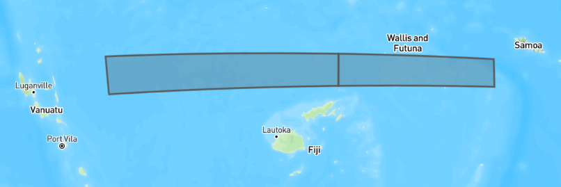
In SeaSketch, the split Polygon will look like this with a line through the middle at -180 or 180 degrees:

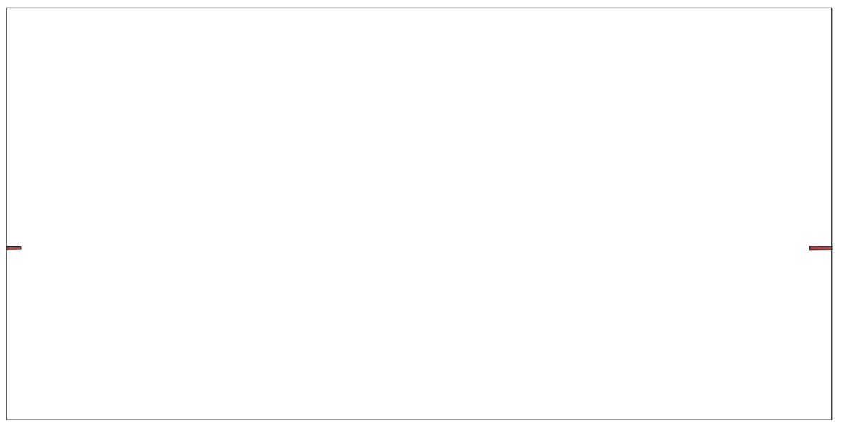
And in GIS software like QGIS, the same split Polygon will look as follows, each half on different sides of the world.
 This is because the portion of the sketch that is "outside", in other words less than 180 degrees, or more than 180 degrees, gets shifted to be within -180 to 180 as part of the splitting process.
SeaSketch doesn't do this split, because it's confusing to the user to see a line split through their Sketch. Geoprocessing functions are left to do this split using the splitSketchAntimeridian() function, which is already included when you use the create:function command.
Just like Sketches, vector datasources that you import and use in preprocessing geoprocessing functions also need to be split. Many global datasources such as OSM land, Marine Regions EEZ, etc. already are split. Other vector datasources are not pre-split and the import CLI command will automatically do this split using the ogr2ogr wrapdateline option.
Raster datasources do not need to be split. They are expected to be within -180 to 180 degrees. This means that data does not go off the left side of the world into less than -180 territory. And data does not go off the right side of the world into greater than 180 territory. So if you have a raster that covers the entire country of Fiji, you will end up with raster cells on both sides of the world, with no data in between. Thankfully, the geoblaze raster analysis library is smart enough to not fetch all the empty data in between when you are analyzing a Sketch that is split onto both sides of the world.

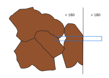
If a Feature or Sketch polygon crosses the antimeridian then so will it's bounding box. And the bounding box of a Sketch is used to fetch from a datasource only the features/raster cells that overlap with that bounding box. And if that bounding box extends across the 180 degree longitude line, then it won't return features or a raster for the portion less than -180, or greater than 180, you will only get the portion inside that range.
Here's an example of a bounding box crossing the Fiji EEZ. The bounding box extends greater than 180, and if you call getFeatures(eezDatasource, bbox) with it you will not get the right side of the Fiji EEZ.

The current (naive) solution is to re-calculate the bounding box after splitting a polygon Sketch. This will produce a bounding box with clean coordinates that are within -180 to 180. The problem is that this produces one long bounding box that extends from -180 all the way to 180. For example, if you take the Fiji bounding box from above and "clean" it, you get the bounding box below. And if you call getFeatures(eezDatasource, cleanBbox) with it, you will get all of the EEZ polygons across that long thin band. This works, if you filter out features after the face, but it is inefficient to send extra features over the network so be careful and watch the execution time of your geoprocessing functions.

A better solution, not yet implemented, would be to split the bounding box into two, just like we do with polygons. You would then need to call getFeatures for each bounding box and de-duplicate where features overlap with both bounding boxes, using a unique ID property.