Vignette guide to the R package
HIVBackCalc estimates HIV incidence, and the number of undiagnosed HIV cases, from testing history data provided by diagnosed cases. The method is based on the basic principle of backcalculation: HIV diagnoses observed in a given year are the convolution of incidence in prior years and the probability of being diagnosed in the given year conditional on infection in a prior year. The package is desgined to be used with HIV surveillance data on the date of diagnosis, and the date of the last negative test for all diagnosed cases in a jurisdiction. Provision is made for cases diagnosed on their first test, and for cases with missing test history data.
This package contains the basic code needed to replicate the analysis in the corresponding paper. However, due to privacy regulations, the dataset included here is a simulated version that matches the population-level characteristics of the original data. The vignette will guide you through a full analysis, with a sensitivity analysis at the end.
The example data embedded in the package approximate testing histories collected from HIV diagnoses among MSM in King County, Washington reported in 2006-2012. The following code will load the data into a data frame called KCsim and display the first 6 rows.
data(KCsim)head(KCsim)| id | Population | mode | race | hdx_age | agecat5 | yearDx | timeDx | everHadNegTest | infPeriod | infPeriod_imputeNA | everHadNegTestM | infPeriodM | |
|---|---|---|---|---|---|---|---|---|---|---|---|---|---|
| 189 | 1 | KC-sim | MSM | Hisp | 35 | 31-35 | 2011 | 2011.25 | TRUE | 0.5315068 | 0.5315068 | FALSE | 18 |
| 483 | 2 | KC-sim | MSM | White | 23 | 21-25 | 2008 | 2008.75 | NA | NA | 7.0000000 | NA | NA |
| 68 | 3 | KC-sim | MSM | Black | 36 | 36-40 | 2009 | 2009.75 | NA | NA | 18.0000000 | NA | NA |
| 484 | 4 | KC-sim | MSM | White | 32 | 31-35 | 2007 | 2007.50 | TRUE | 10.2575342 | 10.2575342 | FALSE | 16 |
| 485 | 5 | KC-sim | MSM | White | 36 | 36-40 | 2007 | 2007.50 | FALSE | 18.0000000 | 18.0000000 | FALSE | 18 |
| 69 | 6 | KC-sim | MSM | Black | 35 | 31-35 | 2008 | 2008.25 | TRUE | 0.7671233 | 0.7671233 | FALSE | 18 |
The necessary variables are:
-
Age at diagnosis (hdx_age)
- In the simulated data set, hdx_age is reported in 5 yr intervals.
-
Year of diagnosis (yearDx)
-
Time of diagnosis (timeDx)
- Defined by the reporting time unit. In the example data, diagnoses are reported quarterly, specified using decimals: 0.00 = Q1 (Jan-Mar), 0.25 = Q2, etc. So someone diagnosed in the third quarter of 2008 would have timeDX = 2008.75.
-
Testing history (everHadNegTest, everHadNegTestM)
- Response to "Have you ever had a negative HIV test?"
- Three possible values: TRUE, FALSE and NA
- The second version has a lower number of repeat testers
-
Time from last negative test to diagnosis (infPeriod, infPeriodM)
- If everHadNegTest=FALSE, imputed as the smaller of 18 years, or hdx_age-16.
- The second version has a correspondingly different set of imputed cases
The remainder of the variables are optional descriptive variables by which the data can be stratified for subgroup analyses. We will use the second versions of the last test and infPeriod variables to examine the impact of the repeat testing fraction on the estimates of undiagnosed cases (at the end of this vignette).
The intervals of the timeDx variable represent the discrete time unit for reporting cases, and determine the finest interval by which we may estimate incidence and undiagnosed counts. In the example data, this interval is a quarter year (0.25). We will store this in an object to use throughout:
diagInterval = 0.25This interval maximizes the use of reported information, and defines the unit of analysis for "undiagnosed HIV." Results will be estimated as undiagnosed counts per quarter. Using quarterly reports implies that a diagnosis made within 3 months of infection is acceptable and contributes no "undiagnosed" time. If we used a longer interval, by re-formatting timeDx, this would modify the meaning of "undiagnosed" accordingly.
The testing history data provides bounds for the possible infection period or "infPeriod" within which infection must have occurred, for all diagnosed cases that have a prior negative test. If a case is diagnosed on their first test, there will be no prior negative test (KCsim$everHadNegTest=FALSE), and we need an alternative approach to defining the possible infection period. In the paper, these cases were assigned an infperiod that was the minimum of 18 years or age-16.
The next step is to aggregate these individual infection periods and use them to define a population level probability distribution for the time from infection to diagnosis (TID). This will require making some assumption regarding when infection occurred within the possible infection period.
HIVBackCalc implements the assumptions that define the two "cases" for the TID examined in the paper:
Base Case - The probability of acquiring infection is uniformly distributed across the infection period. This assumes testing is not driven by risk exposure, so is likely to be conservative (i.e., overestimate the time spent undiagnosed).
Upper Bound - All infections occur immediately after the last negative test. This is an extremely conservative assumption that represents the maximum possible amount of time people could have been infected but undiagnosed.
The estimateTID function will return the probability and cumulative density functions for each of these cases.
TIDs <- estimateTID(KCsim$infPeriod, intLength=diagInterval)We can examine the TID for each case by plotting the probability and survivor functions.
plot(TIDs, intLength=diagInterval,
     cases = c('Base Case', 'Upper Bound'))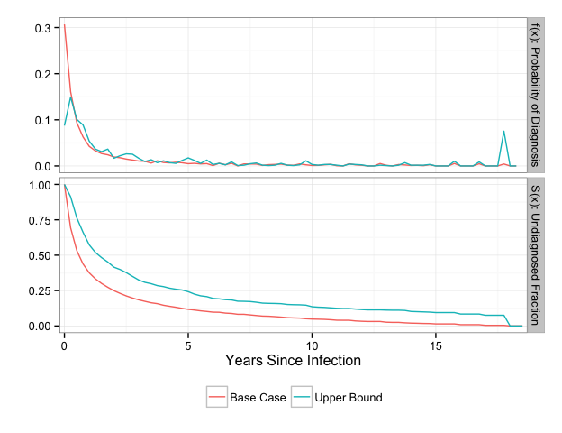
The spike in density at 18 years for the Upper Bound TID reflects the assumption we made for the cases that were diagnosed at their first test.
We can evaluate the TID at particular time points of interest using the summary function. The time points should be specified in years and represent the left bound of the discrete time between infection and diagnosis.
summary(TIDs, intLength=diagInterval,
        cases = c('Base Case', 'Upper Bound'),
times =c(0, 0.25, 1, 5, 10, 18))| Time | Base Case f(x) | Base Case S(x) | Upper Bound f(x) | Upper Bound S(x) |
|---|---|---|---|---|
| 0.00 | 0.3176424 | 0.6823576 | 0.1016419 | 0.8983581 |
| 0.25 | 0.1583612 | 0.5239964 | 0.1469898 | 0.7513683 |
| 1.00 | 0.0419130 | 0.3278006 | 0.0531665 | 0.5113370 |
| 5.00 | 0.0048178 | 0.1106343 | 0.0172009 | 0.2212666 |
| 10.00 | 0.0009740 | 0.0469671 | 0.0031274 | 0.1305708 |
| 17.00 | 0.0000000 | 0.0041226 | 0.0000000 | 0.0742768 |
| 18.00 | 0.0000000 | 0.0000000 | 0.0000000 | 0.0000000 |
To backcalculate incidence, we must define a vector of diagnosis counts per interval. By default, this vector contains 100 empty intervals prior to the first interval in which we observe diagnoses. These empty intervals will indicate to the model how far back to project incidence.
diagCounts = tabulateDiagnoses(KCsim, intLength=diagInterval)The backcalculation uses the same diagnosis counts but different TIDs to project incidence for each of the cases.
incidenceBase = estimateIncidence(y=diagCounts,
                                  pid=TIDs[['base_case']]$pdffxn,
                                  gamma=0.1,
                                  verbose=FALSE)
incidenceUpper = estimateIncidence(y=diagCounts,
                                  pid=TIDs[['upper_bound']]$pdffxn,
                                  gamma=0.1,
                                  verbose=FALSE)
We can plot the backcalculated estimates over time, overlayed by the diagnosis counts in red.
plot(incidenceBase, case='Base Case')
plot(incidenceUpper, case='Upper Bound')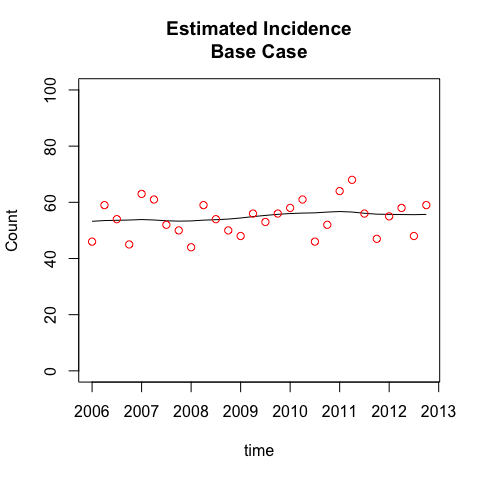
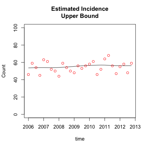
While the TIDs for the two cases are quite distinct, the incidence estimates are almost identical. This is because the diagnosis counts are relatively stable, and the TIDs are constant, not year-specific (this assumption was tested in the paper). Together, this implies that incidence is approximately equal to diagnosed cases, and both TID cases will conform to this incidence estimate. The impact of the different TID assumptions is just to recalibrate the fraction of prevalent infections that are diagnosed at any point in time. People have been undiagnosed for longer in the upper bound case, so the observed diagnoses in this case are estimated to have a greater fraction of persons whose time of infection was further in the past. This in turn will generate a higher fraction of recently infected persons who are undiagnosed, as we see next.
Estimating undiagnosed counts requires applying the TID to the incidence estimates to determine how many of those who were ultimately diagnosed were undiagnosed in a given interval.
# Base Case
undiagnosedBase <- estimateUndiagnosed(incidenceBase)
# Upper Bound
undiagnosedUpper <- estimateUndiagnosed(incidenceUpper)The results of the two cases can be combined and contrasted by creating a "results" object using combineResults(). Note that the names of the upper-level list, e.g. "Base Case" and "Upper Bound", will be used to label the respective results in the results plots and tables that follow.
results <- combineResults(list(`Base Case`=list(incidenceBase,
                                            undiagnosedBase),
                             `Upper Bound`=list(incidenceUpper,
                                              undiagnosedUpper)))
The estimates are summarized over all time periods in the results$resultsSummary element.
results$resultsSummary| Diagnoses/Case | Estimate | Min. | 1st Qu. | Median | Mean | 3rd Qu. | Max. |
|---|---|---|---|---|---|---|---|
| # Diagnosed | Diagnoses | 44.00 | 49.50 | 54.50 | 54.36 | 59.00 | 68.00 |
| Base Case | Incidence | 53.23 | 53.67 | 55.10 | 54.86 | 55.83 | 56.72 |
| Base Case | Undiagnosed Cases | 409.20 | 414.00 | 421.40 | 420.70 | 425.60 | 434.80 |
| Upper Bound | Incidence | 53.61 | 53.95 | 55.86 | 55.34 | 56.31 | 56.88 |
| Upper Bound | Undiagnosed Cases | 807.80 | 816.50 | 828.80 | 826.50 | 834.80 | 844.90 |
Plotting the results object will panel the incidence and undiagnosed estimates with the cases overlayed:
plot(results)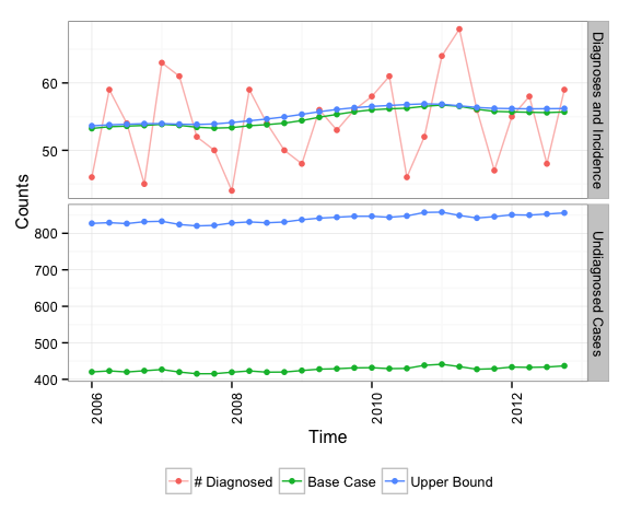
This simpler method may be used if both HIV incidence and the TID probability distribution are constant over time.
We first define incidence as the average of observed diagnoses (per quarter):
constantIncidence <- mean(diagCounts, na.rm=TRUE)We can then apply the TID to estimate undiaagnosed counts assuming this constant incidence:
# Base Case
undiagnosedConstBase <- estimateUndiagnosedConst(infPeriod=KCsim$infPeriod,
                                                 case='base_case',
                                                 intLength=diagInterval,
                                                 incidence=constantIncidence)

# Upper Bound
undiagnosedConstUpper <- estimateUndiagnosedConst(infPeriod=KCsim$infPeriod,
                                                  case='upper_bound',
                                                  intLength=diagInterval,
                                                  incidence=constantIncidence)


rbind(BaseCase=undiagnosedConstBase,
      UpperBound=undiagnosedConstUpper)
## [,1]
## BaseCase 424.1284
## UpperBound 836.8558
In the Seattle/King County jurisdiction, repeat testing among MSM was the norm: over 90% of those with known testing history reported a previous negative test, and the median inter-test interval was just over a year. Our methods perform well in this setting, as the uncertainty is well bounded in the observed data.
In other jurisdictions, repeat testing may be less common, with more people diagnosed on their first test. In this case, the length of the period during which infection may have occurred is not bounded by an observed inter-test interval, it must be imputed, and that requires an assumption.
Our method takes a relatively conservative approach to this imputation, assuming the window of possible infection is the shorter of 18 years, or age-16. The base case estimates assume the probability of infection is uniformly distributed across this interval; the upper bound assumes infection occurs at the beginning. In both cases, this introduces a potentially long period of undiagnosed infection.
To get a sense of how this would affect the estimates of the number of undiagnosed cases, we will analyze the simulated dataset with 50% of the repeat testers randomly recoded to have no previous test. The recoded data are the variables "everHadNegTestM" and "infPeriodM".
We'll run the estimates with the constant incidence assumption, and compare the results.
First, compare the data, before and after the random last negative test deletions:
## Comparing whether last negative test exists

##        FALSE TRUE <NA>
## before   166 1113  243
## after    666  613  243

## Comparing length of possible infection window (years)

##          0   1   2  3  4  5  6  7  8  9 10 11 12 13 14 15 16 17  18 <NA>
## before 318 353 134 98 49 59 34 17 17 12 23 10 12  3 15  6 13 11  95  243
## after  183 186  73 52 21 56 36 47 30 31 41 27 31 22 29 28 31 27 328  243
Roughly half of the non-missing cases are now diagnosed on their first test, and the distribution of the possible infection window is strongly shifted to the right.
constantIncidence <- mean(diagCounts, na.rm=TRUE)

# Base Case
undiagnosedConstBaseM <- estimateUndiagnosedConst(infPeriod=KCsim$infPeriodM,
                                                 case='base_case',
                                                 intLength=diagInterval,
                                                 incidence=constantIncidence)

# Upper Bound
undiagnosedConstUpperM <- estimateUndiagnosedConst(infPeriod=KCsim$infPeriodM,
                                                  case='upper_bound',
                                                  intLength=diagInterval,
                                                  incidence=constantIncidence)
## Compare resulting estimates of the number of undiagnosed cases
## BaseCase UpperBound
## before 424.0 837.0
## after 950.0 1867.0
## ratio 2.2 2.2
The estimate of the number of undiagnosed cases is roughly doubled, for both the base case and the upper bound assumptions. This will also double the estimate of the undiagnosed fraction, because the number of cases is still small relative to the estimated number of persons living with HIV in this setting. Thus, with an increase from 9% to 50% of the diagnoses coming from first-time testers, our estimates of the undiagnosed fraction would increase from the 6-11% range we report in the paper to something on the order of 12-22%.
Of course, many other assumptions could be made about the differences between repeat testers and those diagnosed on their first test. Some of these could lead to different results. For example, if the repeat testers are coming in on a regular annual schedule, while the first-time testers are testing in response to a recent risk exposure, then we would expect little impact on the estimates, or perhaps a small reduction in the undiagnosed fraction. On the other hand, the Upper Bound estimate for the recoded data does give the worst case that is still consistent with the data.