#Title Data Mining 2016 Presidential Campaign Finance Data
#Tags campaign finance, elections, preprocessing, data cleaning, data cleansing, feature engineering, free data, large dataset, government, politics, public data
#Summary Play with campaign finance data while learning how to prepare a large dataset for machine learning by processing and engineering features.
#Description
The experiment works on a 2.5 GB dataset and will take about 20 minutes to run in its entirety.
#Objective Learn how to prepare a dataset for machine learning by creating labels, processing data, engineering additional features, and cleaning the data.
#Data Selection This experiment will be using the campaign finance datasets from the Federal Elections Committee (FEC). Specifically, we will be using the “Contributions by Individuals” dataset for the 2015~2016 election cycle.
Under US Federal law, aggregate donations of $200 or more by an individual must be disclosed. This dataset represents the itemized transactions where individuals donate to the political campaigns of candidates, political action committees (PACs) and/or national party committees.
The individual contribution dataset in this experiment represents a sub-sampled variant of the original ~2.5 GB dataset. The original dataset can be found here and this R script will convert it to CSV to be imported into Azure ML.
#Data Mining Problem This dataset is quite versatile and can be adapted for a host of solutions such as predicting the passage of bills, ideaologies of American lawyers, predicting congressional votes, or the probability that a transaction is going towards democrate or republican.
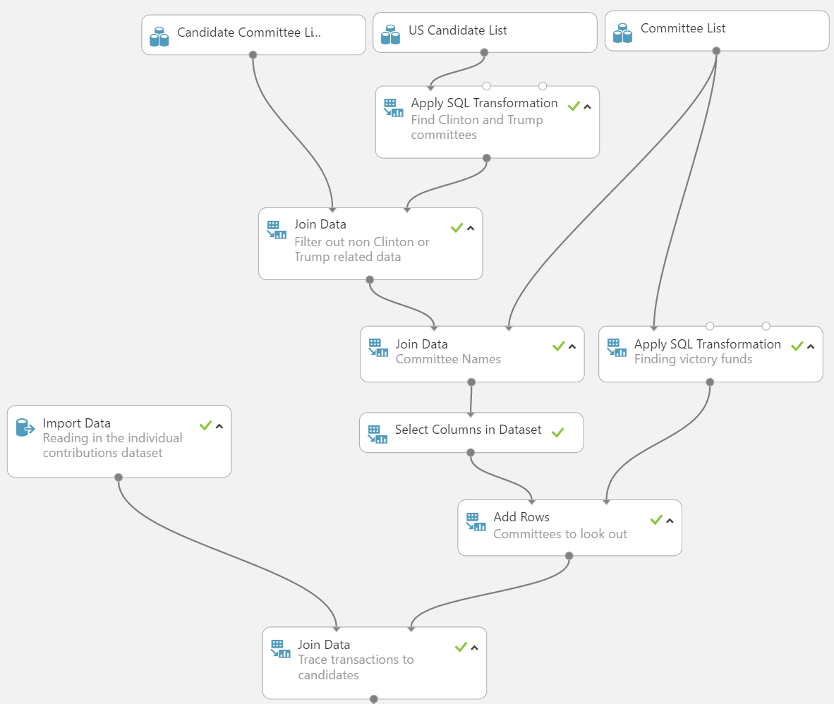
In the spirit of the election, let’s setup the dataset in a way to identify transactions to Hillary Clinton or Donald Trump. To do that we will need to identify and label each transaction (supervised learning) that went toward Clinton or Trump. From then it can become a classification machine learning problem. The individual transactions dataset also contains transactions to all Senators, all House of Representatives, and all Presidential candidates running for election. Those will have to be filtered out, which will be explained in the next section.
#Pulling in Reference Data We will use the committee linkage file which shows the existing relationships between committees to candidates (if a relationship exists) by “candidate id” and “committee id”. There also exists a candidate master file which lists out every candidate by “candidate id”. Lastly there is a committee list that lists out every committee by “committee id”.

Keep in mind that we are ignoring more complex transactions to Clinton and Trump such as JFC funds, DNC or RNC contributions, or non-officially affiliated committees.
 #Feature Engineering Gender
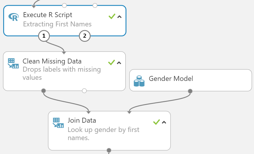
The individual contributions dataset contain full names of each contributor. With this we can pull in data from the Social Security Administration's baby names dataset to predict genders by first names. We will use [R to extract first names and titles](https://github.com/datasciencedojo/DataMiningFEC/blob/master/5 Extracting First Names.R) then cross reference the extracted values in the gender model to derive gender using the join module.
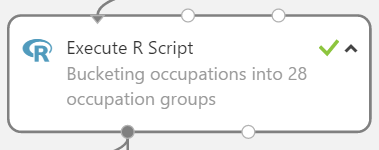
- Occupation: this column represents people’s jobs. People were allowed to fill in this field themselves, free-form. As a result, there are a large number of misspellings. The word “veteran” can also be found as “veteren”, “WWII vet” and “vetren”. As a result, there are 33,507 distinct occupations our dataset. Luckily the Bureau of Labor Statistics has done by classifying each job title into one of 28 occupational type buckets for us. We wrote an [R script](https://github.com/datasciencedojo/DataMiningFEC/blob/master/6 Bucketing Occupation Groups.R) in Azure ML to do this bucketing.
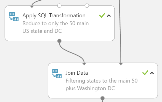
- State: there are 60 states in this dataset; 50 main US States, Washington DC, and 9 extra states. The extra 9 states represent overseas military bases, citizens working abroad, or other territories such as Pacific Islands. However, these extra 9 states also only account for 4151 rows, which is less than half a percent of data which means there may not be enough representation to learn from these categories. We will use a SQL statement to filter out only the 50 main states plus Washington DC.
- Cities: there are 11,782 distinct city names. We will run a SQL query to filter out city and state combinations that don’t have at least 50 transactions. We filter these out because there are not enough observations to form representation within the dataset. This threshold becomes a tuning parameter that you can play with. Increasing it may improve the overall performance of your models at the cost of less granularity for the inclusion of a specific city. After the filtering, 2,489 cities remain.
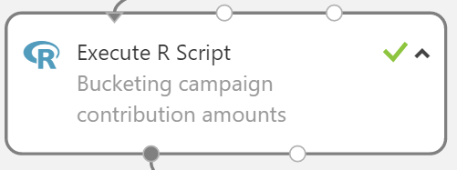
- Contribution amounts: this feature does not have to be bucketed. However, in the experiment, we show that you can bucket numeric features by quantile percentages.
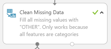
#Cleaning Missing Data All columns have missing values. For simplicity all missing values were replaced with a separate category called “OTHER”. However, it is advised at this step to experiment with different methods of missing value cleansing to see if there is a performance increase.
Note that any rows containing missing values of the response label have to be removed because supervised learning models can only learn if there is a label present for a given row.
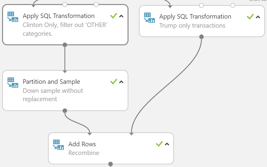
#Dealing with Class Imbalance There is a steep asymetric between the class labels, whereas Clinton transactions (94%) are way more common than Trump transactions (6%). Class imbalance is quite common in machine learning, where one class is rarer than another. Some examples include medical diagnosis of tumor cells, a certain hormone that signifies pregnancy, or a fraudulent credit card transaction. There are many ways to combat class imbalance, however the one that is employed here will be to down sample the common class or to oversample the rare class. Clinton’s transactions were randomly sampled down (7%) to match Trump’s 58k transactions. This sampling percentage also becomes a tuning parameter for future predictive models.
#Next Steps The data should be in a state where it can be fed into one of many machine learning algorithms to build a model. There were also a lot of features dropped that would be ripe for feature engineering further. For example, the “memo” column contains important clarification on each transactions such as if the transaction was a refund, an earmark, and other interesting items. Research and extracting into this column can yield a more granular dataset for the model. The “image number” column also contains within it month and day of the receipt’s scan. Extracting day of the week can yield other interesting features such as whether or not it’s a holiday or not.
- Detailed Tutorial: Building and deploying a classification model in Azure Machine Learning Studio
- Demo: Interact with the user interface of a model deployed as service
- Tutorial: Creating a random forest regression model in R and using it for scoring
- Tutorial: Obtaining feature importance using variable importance plots
