-
Notifications
You must be signed in to change notification settings - Fork 41
Plotter
Some classes are provided to facilitate making plots in CMS style.
If you have a list of histograms, hists, you want to compare with a ratio plot,
use the Plot class, e.g.
from TauFW.Plotter.plot.Plot import Plot, CMSStyle
CMSStyle.setCMSEra(2018)
plot = Plot("x",hists)
plot.draw(ratio=True,grid=True,logy=True)
plot.drawlegend()
plot.saveas("plot.png")
plots.close()
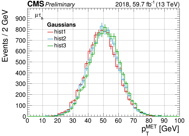
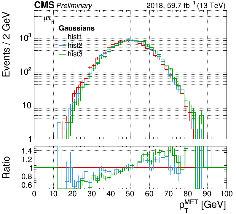
If you want to make a data-MC comparison between a data histogram datahist and
a list of expected SM processes, exphists,
you can use the Stack class, with something like
from TauFW.Plotter.plot.Stack import Stack, CMSStyle
CMSStyle.setCMSEra(2018)
plot = Stack("p_{T} [GeV]",datahist,exphists)
plot.draw(ratio=True,logy=False)
plot.drawlegend(pos='right')
plot.drawtext("#mu#tau_{h} baseline")
plot.saveas("stack.png")
plot.saveas("stack.pdf")
plots.close()
You can create 2D histograms using the Plot2D class, e.g.
from TauFW.Plotter.plot.Plot2D import Plot2D
CMSStyle.setCMSEra(2018)
plot = Plot2D("x","y",hist)
plot.draw(logz=True,ztitle="Events")
plot.drawlegend()
plot.drawtext("#mu#tau_{h} baseline")
plot.drawprofile('x')
plot.saveas("plot2D.png")
plots.close()
Simple examples of usage of Plot and Stack are provided in test/, run as
test/testPlot.py -v2
test/testStack.py -v2
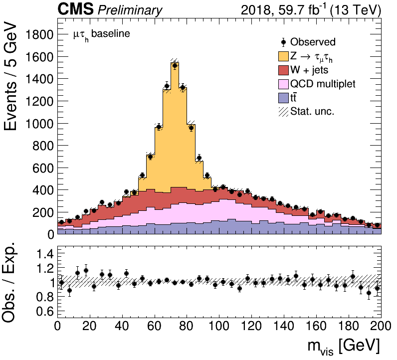
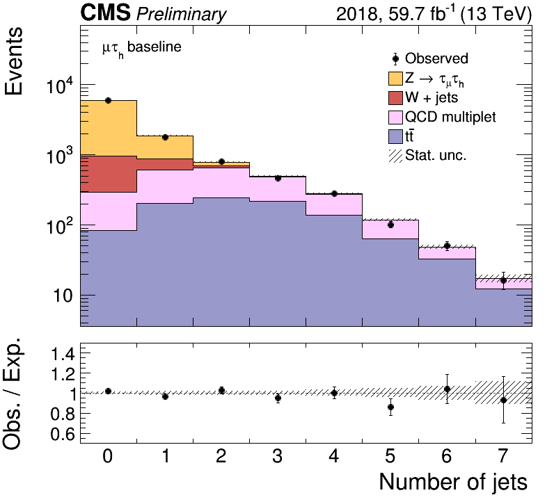
CMSStyle.py provides tools to make a plot have the CMS style.
The integrated luminosity and center-of-mass energy are automatically set for a given year with hardcoded defaults.
For example,
CMSStyle.setCMSEra(2018)
will set 59.8 fb^{#minus1} in all plots.
You can change the defaults with keyword arguments like
CMSStyle.setCMSEra(2018,lumi=59.7,cme=13,cms="CMS",extra="Preliminary")
Or you can directly change the hardcoded default values for your own plotting script as follows:
import TauFW.Plotter.plot.CMSStyle as CMSStyle
CMSStyle.cmsText   = "CMS"
CMSStyle.extraText = "Preliminary"
CMSStyle.lumi_dict['UL2018'] = 59.8
CMSStyle.lumi_dict['UL2018'] = 59.8
CMSStyle.era_dict['UL2018'] = "2018"
Note that there is also the function setera, which is used to set the global luminosity for the normalization to cross section times integrated luminosity for all MC samples, and which calls CMSStyle.setCMSEra to set the default plotting labels. It is explained in more detail below.
A Variable class is provided to contain variable name (e.g. pt_1),
title (e.g. Leading p_{T} [GeV]) and the binning (nbins,xmin,xmax or a list of bins edges), for example:
from TauFW.Plotter.plot.Variable import Variable
variables = [
  Variable('pt_1',  "p_{T}",   40, 0,200),
  Variable('m_vis', "m_{vis}", [0,20,40,50,60,65,70,75,80,85,90,100,120,150]),
  Variable('njets', "Number of jets", 8, 0,  8),
  Variable('nbtag', "Number of b jets", 8, 0,  8, weight="btagweight"),
  Variable('pt_1+pt_2+jpt_1', "S_{T}", 40, 0, 800, cut="jpt_1>50", fname="ST"),
]
A Variable object can contain a lot of information, passed as key-word arguments that are
useful when making plots (e.g. ymin, ymax, logx, logy, ymargin, ...)
or selection strings (e.g. cut, blind, weight, ...).
It also has several handy functions that provide shortcuts for common routines.
For example, Variable.gethist can create a histogram for you:
hist = var.gethist()
and Variable.drawcmd can parse a draw command for TTree::Draw:
var  = Variable('pt_1',40,0,200)
hist = var.gethist('hist') # returns a TH1D with name 'hist'
dcmd = var.drawcmd('hist') # returns a string, e.g. "pt_1 >> hist"
tree.Draw(dcmd)            # loops over tree events and fills the histogram 'hist'
It can also be used to initialize a Plot, Plot2D, or Stack object, e.g.
xvar = Variable('pt_1',40,0,200,logy=True,ymargin=1.4)
yvar = Variable('pt_1',40,0,200,logy=True,ymargin=1.4)
plot = Plot(xvar,hists)
plot2D = Plot2D(xvar,yvar,hist2D)
Examples are provided in test/testVariables.py.
Often, plots need to be adjusted for different selections.
You might need a larger range at higher energies, or a wider binning for fewer events.
To avoid cluttering code with a bunch of if statements. the Variable class offers a way
to change things like the binning, title, extra cuts, etc. on the context.
The context can be triggered by a set of strings.
To change the binning, specify the context for example the cbin option:
var = Variable('pt_1',"pt",40,0,200,cbin={'nbtag>=1':(50,0,500)}),
for sel in ["pt_1>30","pt_1>50 && nbtag>=1"]:
  var.changecontext(sel)  # check if string matches a predefined context
  hist = var.gethist()    # binning will depend on the context
Here, cbin is a dictionary whose keys are regular expression that are matched to strings passed
to Variable.changecontext. If the string matches a predefined key ('nbtag>=1' in the case above),
the associated binning is used.
If there are multiple keys, they are ordered by length, from most to least number of characters.
The longest strings that matches will be used.
Similarly, one can change the title using ctitle, e.g.
var = Variable('pt_1',"Muon pt",40,0,200,ctitle={'etau':"Electron pt",'tautau':"Tau pt"}),
for channel in channels:
  for sel in selections:
     var.changecontext(channel,sel)
To see how this works in action, please play around with test/testVariables.py.
A Sample class is provided to contain and interface your analysis ntuples (pico).
It keeps track of a sample's information like title (for legends), filename, cross section, normalization, etc.
To initialize, you need to pass a unique name, a title (for legends) and a filename:
sample = Sample("TT","t#bar{t}","TT_mutau.root",831.76)
The fourth argument can be a float that is the cross section (in units of pb).
It will be used by Sample.normalize to compute the normalization to the integrated luminosity times cross section as
norm = lumi*xsec*1000/sumw
if the total sum of weights, sumw, of all MC samples is given, otherwise the total number of MC events nevts is used.
The total number of events and total sum of weights will automatically be taken from the
'cutflow' histogram if it exists,
otherwise, the user should pass it directly with nevts or sumw:
sample = Sample("TT,"t#bar{t}","TT_mutau.root",831.76,nevts=76915549,lumi=59.7)
Instead of passing the integrated luminosity with lumi (in units of inverse fb) to Sample, you can set it globally
in python/sample/utils.py by passing the era like this:
from TauFW.Plotter.sample.utils import setera
setera(2018)
This will also immediately set the era for plots via CMSStyle. To set the era manually,
directly edit the dictionary lumi_dict in the python/sample/utils.py, or use
setera(2018,59.7)
Sample provides a useful method that can create and fill a histogram (TH1D) for some variable.
It can be called in several ways:
var  = Variable('m_vis',40,0,200)
hist = sample.gethist('m_vis',40,0,200,"pt_1>30 && pt_2>30")
hist = sample.gethist('m_vis',[0,40,50,60,70,90,100,120,200],"pt_1>30 && pt_2>30")
hist = sample.gethist(var,"pt_1>30 && pt_2>30")
To speed up things, it can create histograms in parallel with RDataFrame:
vars = [
  Variable('m_vis', 40,0,200),
  Variable('nbtags', 8,0,  8, weight="btagweight"),
  Variable('jpt_1', 40,0,200, cut="abs(jeta_1)<2.5", title="Forward jet pt"),
]
hists = sample.gethist(vars,"pt_1>30 && pt_2>30")
where vars is a list of variables as above, and the returned hists is a list of TH1Ds.
Similarly, Sample.gethist2D is available for 2D histograms (TH2D).
With Variable objects, you can include extra cuts or weights that are variable-specific.
In the example above, the btagweight weight will only be applied to nbtags,
and the jpt_1>0 cut only to jpt_1.
You can also split samples into different components (e.g. real/misidentified, or decay mode) based on some cuts. e.g.
sample.split(('ZTT',"Real tau","genmatch_2==5"),
             ('ZJ', "Fake tau","genmatch_2!=5"))
hists = { }
for subsample in sample.splitsamples:
  hists[subsample] = subsample.gethist(vars,"pt_1>50")
Each component is defined by a unique name (e.g. 'ZTT' and 'ZJ'), a title "Real tau", and a cut,
which must be orthogonal to the others to avoid overlap.
Examples are provided in test/testSamples.py:
test/testSamples.py -v2
The color and title style is predefined by dictionaries in python/sample/SampleStyle.py.
These dictionaries are used to automatically set the color for Sample object if none is passed.
You can change the default sample colors and title to your preference as
import TauFW.Plotter.sample.SampleStyle as STYLE
STYLE.sample_colors['ZTT'] = kOrange-4
STYLE.sample_titles['ZTT'] = "Z -> #tau#tau
Some string patterns for axis titles and legend entries are automatically converted to LaTeX format
by makelatex in python/plot/string.py. To disable this, pass the latex=False
option to the Plot.draw, Plot.drawlegend and , Plot.drawtext functions.
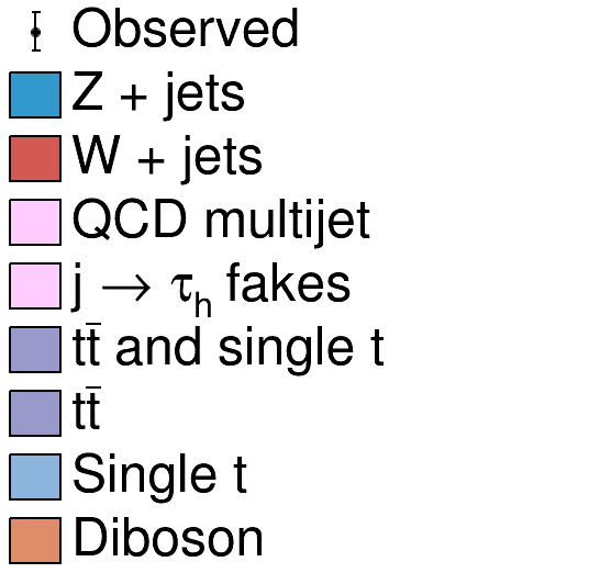
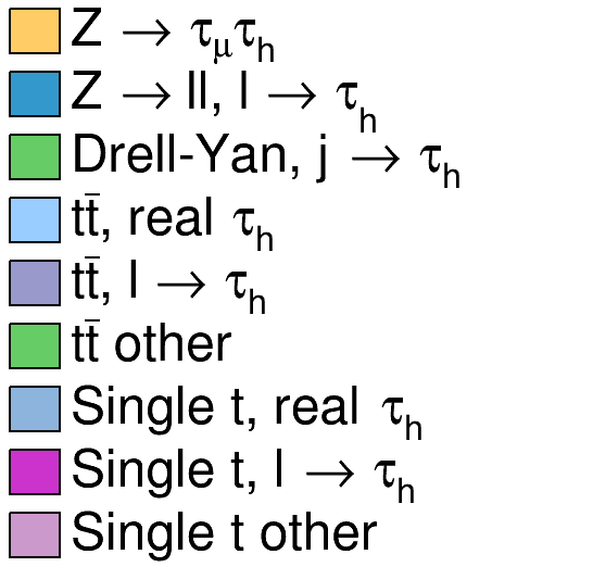
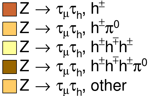
The SampleSet class helps to contain data and MC Samples objects:
from TauFW.Plotter.sample.SampleSet import SampleSet
samples = SampleSet(datasample,expsamples)
samples.printtable()
Here, datasample is a single Sample object of observed data,
while expsamples is a simple python list of Sample objects wrapping MC ntuples.
To make initialization of sample sets of pico ntuples easier,
you can use the help function getsampleset, for example:
expsamples = [ # table of MC samples to be converted to Sample objects
  ('DY', "DYJetsToLL_M-10to50",  "Drell-Yan 10-50", 18610.0, {'extraweight': 'zptweight'} ),
  ('WJ', "WJetsToLNu",           "W + jets",        50260.0, ),
  ('TT', "TT",                   "ttbar",             831.76 ),
]
datasamples = ('Data', "SingleMuon_Run2016?", "Observed") # to be converted to Sample object
sampleset = getsampleset(datasamples,expsamples,era=2016)
Here, expsamples is a list of python tuples:
( GROUP, SAMPLE, TITLE, XSEC )
To pass special options via keywords, use an extra dictionary.
Here, group name GROUP and sample name SAMPLE correspond to what was used during pico production.
Data is a single tuple:
( GROUP, SAMPLE, TITLE )
Here, SAMPLE should be the data set name (e.g. SingleMuon_Run2016) corresponding to a single pico file
(e.g. SingleMuon_Run2016_mutau.root) containing processed events of the whole data period,
or it can be a pattern (e.g. SingleMuon_Run2016?) for multiple files
(e.g. SingleMuon_Run2016B_mutau.root, SingleMuon_Run2016C_mutau.root, ...)
By default, getsampleset will automatically assume the samples can be found via the pattern
"$PICODIR/$SAMPLE_$CHANNEL.root"
where PICODIR will be retrieved from the PicoProducer config file.
You can instead specify to getsampleset the file name pattern with the keyword file.
With the keyword option url you can pass a XRootD url that will be prepended to this pattern.
To get an overview of the samples, use
sampleset.printtable()
>>> Samples with integrated luminosity L = 35.9 / fb at sqrt(s) = 13 TeV
>>> Sample name                title                      xsec [pb]      nevents    sumweights      norm  weight
>>> SingleMuon_Run2016         Observed                                                            1.000
>>> ├─ SingleMuon_Run2016B     Observed                       -1.00  154054252.0  154054252.00     1.000
>>> ├─ SingleMuon_Run2016C     Observed                       -1.00   64718679.0   64718679.00     1.000
>>> ├─ SingleMuon_Run2016D     Observed                       -1.00   96657799.0   96657799.00     1.000
>>> ├─ SingleMuon_Run2016E     Observed                       -1.00   87378748.0   87378748.00     1.000
>>> ├─ SingleMuon_Run2016F     Observed                       -1.00   65047318.0   65047318.00     1.000
>>> ├─ SingleMuon_Run2016G     Observed                       -1.00  147941144.0  147941144.00     1.000
>>> └─ SingleMuon_Run2016H     Observed                       -1.00  171137991.0  171137991.00     1.000
>>> DYJetsToLL_M-50            Drell-Yan 50                 4963.00  146280395.0  146277764.00     1.218  zptweight
>>> WJetsToLNu                 W + jets                    50260.00   86413370.0   86411825.00    20.880
>>> TT                         ttbar                         831.76   76915549.0   76914152.00     0.388  ttptweight
The luminosity-cross section normalization is given by the norm column, which is described above.
A full example is given in test/plotPico.py.
This script assumes a complete list of 2016 pico ntuples in the mutau channel.
Sometimes you want to group samples into one bigger merged sample,
to reduce the number of backgrounds on your plots, or treat them as one in a fit.
This can be done with by using the MergedSample class,
but SampleSet provides a help function that does it for you, for example,
sampleset.join('DY',               name='DY', title="Drell-Yan"           )
sampleset.join('VV','WZ','WW','ZZ',name='VV', title="Diboson"             )
sampleset.join('TT','ST',          name='Top',title="ttbar and single top")
The name and (legend) title of the merged sample is passed by the keyword arguments name and title.
The first string arguments are different search terms or glob patterns (with * wildcards) that can be used to identify the samples you want to merge.
In the TauPOG, typically "jet-binned" samples of Drell-Yan (Z+jets) and W+jets are used,
like DY[1-4]JetsToLL_M-50* or W[1-4]JetsToLNu*. (Here "jet" means number of LHE-level partons.)
They increase the statistics, but overlap with their respective jet-inclusive sample.
Therefore a special "stitching" procedure is needed that changes the effective
luminosity-cross section normalization per "jet-bin", before they are merged into one big sample.
The method is explained on this TWiki page.
You can use the stitch help function to do it automatically:
sampleset.stitch("W*Jets",   incl='WJ', name='WJ'                               )
sampleset.stitch("DY*J*M-50",incl='DYJ',name="DY_M-50",title="Drell-Yan M=50GeV")
Again, the first strings arguments are search terms or patterns to identify the samples you want to stitch together.
The keyword argument incl is the search term to identify the inclusive samples (e.g. DYJetsToLL_M-50 or WJetsToLNu).
As per HTT convention, the branch variable name that indicates the number of partons ("jets") is called NUP.
This variable corresponds to LHE_Njets in nanoAOD.
To understand how the normalization is computed, look in python/sample/utils.py,
and pass stitch the option verbosity=2 to printout a table.
The k-factor is computed on the fly. You can set the (N)NLO cross section via the xsec keyword,
or by changing the hardcoded xsecs_nlo dictionary in utils.py.
In the end, after merging and stitching, you might obtain something a summary table like this:
sampleset.printtable()
>>> Samples with integrated luminosity L = 35.9 / fb at sqrt(s) = 13 TeV
>>> Sample name                title                      xsec [pb]      nevents    sumweights      norm  weight
>>> SingleMuon_Run2016         Observed                                                            1.000
>>> ├─ SingleMuon_Run2016B     Observed                       -1.00  154054252.0  154054252.00     1.000
>>> ├─ SingleMuon_Run2016C     Observed                       -1.00   64718679.0   64718679.00     1.000
>>> ├─ SingleMuon_Run2016D     Observed                       -1.00   96657799.0   96657799.00     1.000
>>> ├─ SingleMuon_Run2016E     Observed                       -1.00   87378748.0   87378748.00     1.000
>>> ├─ SingleMuon_Run2016F     Observed                       -1.00   65047318.0   65047318.00     1.000
>>> ├─ SingleMuon_Run2016G     Observed                       -1.00  147941144.0  147941144.00     1.000
>>> └─ SingleMuon_Run2016H     Observed                       -1.00  171137991.0  171137991.00     1.000
>>> DY                         Drell-Yan                                                           1.000
>>> ├─ DYJetsToLL_M-10to50     Drell-Yan 10-50             18610.00   35114961.0   35114342.00    19.026  zptweight
>>> └─ DY_M-50                 Drell-Yan M=50GeV                                                   1.000
>>>    ├─ DYJetsToLL_M-50      Drell-Yan 50                 4963.00  146280395.0  146277764.00     1.000  zptweight
>>>    ├─ DY1JetsToLL_M-50     Drell-Yan 1J 50              1012.00   63730337.0   63729233.00     0.476  zptweight
>>>    ├─ DY2JetsToLL_M-50     Drell-Yan 2J 50               334.70   19879279.0   19878905.00     0.495  zptweight
>>>    ├─ DY3JetsToLL_M-50     Drell-Yan 3J 50               102.30    5857441.0    5857336.00     0.507  zptweight
>>>    └─ DY4JetsToLL_M-50     Drell-Yan 4J 50                54.52    4197868.0    4197790.00     0.413  zptweight
>>> WJ                         W + jets                                                            1.000
>>> ├─ WJetsToLNu              W + jets                    50260.00   86413370.0   86411825.00     1.000
>>> ├─ W1JetsToLNu             W + 1J                       9625.00   43773492.0   43772700.00     7.012
>>> ├─ W2JetsToLNu             W + 2J                       3161.00   60366929.0   60365816.00     2.111
>>> ├─ W3JetsToLNu             W + 3J                        954.80   59300029.0   59298987.00     0.689
>>> └─ W4JetsToLNu             W + 4J                        494.60   29941394.0   29940855.00     0.706
>>> VV                         Diboson                                                             1.000
>>> ├─ WW                      WW                             75.88    7982180.0    7982164.32     0.341
>>> ├─ WZ                      WZ                             27.60    3997571.0    3997499.00     0.248
>>> └─ ZZ                      ZZ                             12.14    1988098.0    1988063.00     0.219
>>> Top                        ttbar and single top                                                1.000
>>> ├─ ST_t-channel_top        ST t-channel t                136.02   31848000.0   31835196.51     0.153
>>> ├─ ST_t-channel_antitop    ST t-channel at                80.95   17780700.0   17771156.67     0.164
>>> ├─ ST_tW_top               ST tW                          35.85    4983500.0  173905506.74     0.007
>>> ├─ ST_tW_antitop           ST atW                         35.85    4980600.0  174107294.88     0.007
>>> └─ TT                      ttbar                         831.76   76915549.0   76914152.00     0.388  ttptweight
This is the output of the full example given in test/plotPico.py.
This script assumes a complete list of 2016 pico ntuples in the mutau channel.
Like described above, you can split samples via SampleSet:
sampleset.split('DY',[
  ('ZTT',"Z -> tau_{#mu}tau_{h}",      "genmatch_2==5"),
  ('ZL', "Drell-Yan with l -> tau_{h}","genmatch_2>0 && genmatch_2<5"),
  ('ZJ', "Drell-Yan with j -> tau_{h}","genmatch_2==0")
])
The SampleSet class can create and fill histograms for you:
result = samples.gethists(var,selection)
print(result.var)                # Variable
print(result.data)               # TH1D
print(result.exp)                # list of TH1Ds
var, datahist, exphists = result # Variable, TH1D, list
Or with for a list of variables to fill histograms in parallel:
result = samples.gethists(vars,selection)
print(result.vars)               # list of Variable
print(result.data)               # dictionary of Variable object to TH1D
print(result.exp)                # dictionary of Variable object to list of TH1Ds
for var, datahist, exphists in result:
  print(var, datahist, exphists) # Variable, TH1D, list
Here, result is a HistSet object, which contains a list of Variable objects,
and dictionaries for data and MC histograms.
Alternatively, you can immediately prepare the histograms into a Stack plot:
stacks = samples.getstack(variables,selection)
for stack in stacks:
  stack.draw()
  stack.drawlegend()
  stack.saveas()
  stack.close()
Examples are provided in test/testSamples.py.
Data-driven background methods like QCD or j → 𝜏h fake estimation can be added as plug-ins
in python/methods/. A python file should contain a function of the same name,
e.g. for the QCD_OSSS.py example:
from TauFW.Plotter.sample.SampleSet import SampleSet
def QCD_OSSS(self, variables, selection, **kwargs):
  ...
  return qcdhists
SampleSet.QCD_OSSS = QCD_OSSS # add as class method of SampleSet
The method returns a list of TH1 histograms that correspond one-to-one to the list of variables.
These histograms are subsequently inserted in the list of MC histograms.
To use them, specify the method name when using SampleSet.getstack or SampleSet.gethists:
stacks = samples.getstack(variables,selection,method='QCD_OSSS')
This will load the file and make the method available.
You can set the position of the new histogram in the stack via imethod,
where 0 means on the top, and -1 means on the bottom.
An example of a plotting script for data/MC comparisions is given by plot.py.
It can be run for a given channel and era as
./plot.py -c mutau -y 2018
It will load a SampleSet from config/samples.py as a function of a channel and era.
By default the script will look for pico samples in $PICODIR, specified in the PicoProducer config.
You can edit the scripts and this config file to your specifications and liking.
You can specify what set of selections to apply and what variable to draw by running, for example:
./plot.py -y 2018 -c mutau -S baseline -V m_vis
where baseline is the name of a set of selections defined in the config/setup_mutau.py.
WARNING: If you are using py3, run with the --serial option:
./plot.py -y 2018 -c mutau --serial
Similarly, plot_v10.py produces the same useful plots as plot.py but loads the SampleSet from config/samples_v10.py designed ofr nanoV10 samples.
An example of a 2D plotting script is given by plot2D.py.
It creates 2D histograms for a specified samples. The samples are defined in config/samples.py.
Edit the desired variable pairs and selections in the script, and run for example as
./plot2D.py -c mutau -y 2018 -s DY
Several macros with help functions are provided in python/macros/
and python/corrections/.
Their functions can be loaded using ROOT directly, e.g.
from ROOT import gROOT
gROOT.ProcessLine(".L python/corrections/tauIDSF.C+O")
or via the help function loadmacro as
from TauFW.Plotter.sample.utils import loadmacro
loadmacro("python/corrections/tauIDSF.C")
After that, it can be imported from ROOT
from ROOT import loadTauIDSF, getTauIDSF
loadTauIDSF("sfs.root",'Medium')
sf = getTauIDSF(dm,genmatch)
or used as in variable, selection or weight expressions
in TTree::Draw or RDataFrame (including via Sample.gethist).
Some examples of usage are shown in test/testMacros.py.